Baseline models
Contents
- Data processing
- Baseline Logistic Regression model
- Comparison of different classification methods for baseline model
- More parameter tuning for GBM and SVC methods
- Full model with all features
- XGBoost model
This section considers a number of different methods to predict if a subject has Alzheimer’s disease (AD) or mild cognitive impairment (LMCI). The data used to construct the models is limited to ADNI 1 baseline observations.
A wide range of methods are considered to determine if certain methods are more effective in predicting Alzheimer’s diagnosis. The strategy to evaluate the performance of the different methods is two-fold: First a range of different models are fit on a set of 15 features from the ADNI merge dataset that are known to be important predictors. The best methods identified from this stage are then further investigated on the full set of features.
Data processing
The first section includes a number of data processing steps to transform the pre-processed dataset with all the relevant features from the ADNI database such that different machine learning models can easily be fit on the data.
Data processing steps
- Data and metadata files are imported
- Observations are subset to only include baseline observations for ADNI 1 subjects
- Response and list of predictors to include in baseline model are specified
- Data is split into train and test datasets
- Predictors with missing values for more than 90% of observations are dropped
- Missing values are imputed using a k-means clustering approach (more detail below)
- Predictors are scaled to have zero mean and unit variance
Training and validation approach
The entire dataset with baseline observations for ADNI 1 subjects are split into a 70% training set with 30% of the data held out for validation and testing. Given the limited amount of observations (~800), we decided not keep a second test set to test out-of-sample performance on the final model although this would be have been ideal.
Missing data strategy
The strategy for dealing with missing data has several components. Firstly, the project design ensures consistency of coverage across the different features as we are only considering observations from a single collection protocol (i.e. ADNI 1) and issues with missing data over multiple visits are addressed by only considering baseline visits. The remaining missing observations in the base dataset is dealt with my either dropping the feature if it contains a very large proportion of missing values or using the k-means imputation approach. Excluding features with a very high proportion of missing values is reasonably as they are unlikely to add significant power to the models. The k-means imputation approach, builds on standard mean imputation by running a clustering algorithm on the features to group ‘similar’ observations together and then using the mean within each cluster rather than the overall mean.
Standardizing predictors
Predictors were standardized to have zero mean and unit variance so that methods that are not invariant to scale (e.g. SVM and Lasso Regression) could easily be compared on the same dataset.
Baseline features
The following 15 features included in ADNI merge datset that are known to be important predictors are considered in the simple baseline model:
- Risk factors: AGE, PTEDUCAT, APOE4
- Cognitive tests: ADAS11, ADAS13, MMSE, RAVLT_immediate
- MRI measures: Ventricles, Hippocampus, WholeBrain, Entorhinal, Fusiform, MidTemp, ICV
- Pet measures: FDG
Baseline Logistic Regression model
First a simple Logistic Regression model is fit using the 15 baseline features identified above. The purpose of this model is to provide some initial understanding of the type of accuracy that can be achieved using a small number of features that are expected to be important and a standard modelling method. Some diagnostics are also produced to identify the most important features in the model.
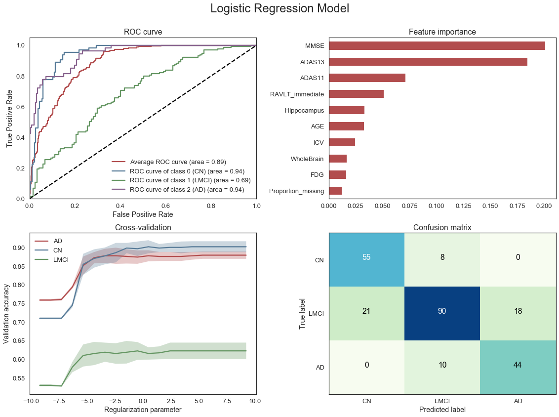
From the diagnostics above we note that the Logistic regression model is able to achieve an average area under the curve (AUC) of 0.88. The model is reasonably effective at correctly identifying true Cognitively Normal (CN) and Alzheimer’s (AD) patients with a fair amount of uncertainty when classifying subjects with Mild Cognitive Impairment (LMCI). The most important features are the cognitive tests followed by some of the MRI measures.
Comparison of different classification methods for baseline model
Next a number of different methods are evaluated on the same set of features used to create the Logistic Regression model above. The following methods are considered with some basic parameter tuning using 10-fold cross validation
- Logistic Regression
- Ridge Regression
- Elastic Net
- K-Nearest Neighbors (KNN)
- Linear Discriminant Analysis (LDA)
- Quadratic Discriminant Analysis (QDA)
- AdaBoost
- Gradient Boosting Method (GBM)
- Support Vector Machines (SVC)
The Elastic Net method was not covered directly in the course. It is a regularized regression method with a penalty term based on weighted L1 and L2 norms. It is therefore effectively weighting the Lasso and Ridge regression methods with the optimal weight determined through cross-validation.
| estimator | min_score | mean_score | max_score | std_score | C | gamma | kernel | l1_ratio | learning_rate | n_estimators | n_neighbors | |
|---|---|---|---|---|---|---|---|---|---|---|---|---|
| 13 | RF | 0.7143 | 0.7834 | 0.8621 | 0.0485 | - | - | - | - | - | 50 | - |
| 19 | GBM | 0.7321 | 0.7800 | 0.8621 | 0.0439 | - | - | - | - | 0.05 | 50 | - |
| 28 | SVC | 0.6724 | 0.7784 | 0.8621 | 0.0580 | 1 | - | linear | - | - | - | - |
| 9 | LDA | 0.6724 | 0.7764 | 0.8966 | 0.0621 | - | - | - | - | - | - | - |
| 29 | SVC | 0.6724 | 0.7715 | 0.8621 | 0.0586 | 10 | - | linear | - | - | - | - |
| 14 | RF | 0.6964 | 0.7711 | 0.8621 | 0.0416 | - | - | - | - | - | 100 | - |
| 15 | RF | 0.6786 | 0.7711 | 0.8793 | 0.0606 | - | - | - | - | - | 500 | - |
| 0 | LogisticRegression | 0.6552 | 0.7697 | 0.9138 | 0.0707 | - | - | - | - | - | - | - |
| 12 | RF | 0.7143 | 0.7662 | 0.8182 | 0.0367 | - | - | - | - | - | 20 | - |
| 20 | GBM | 0.6491 | 0.7660 | 0.8448 | 0.0577 | - | - | - | - | 0.05 | 100 | - |
The table above ranks the methods with relevant hyper-parameters by mean validation accuracy. We note that the mean accuracy based on a 10-fold cross-validation of the first 5-6 models are very similar.
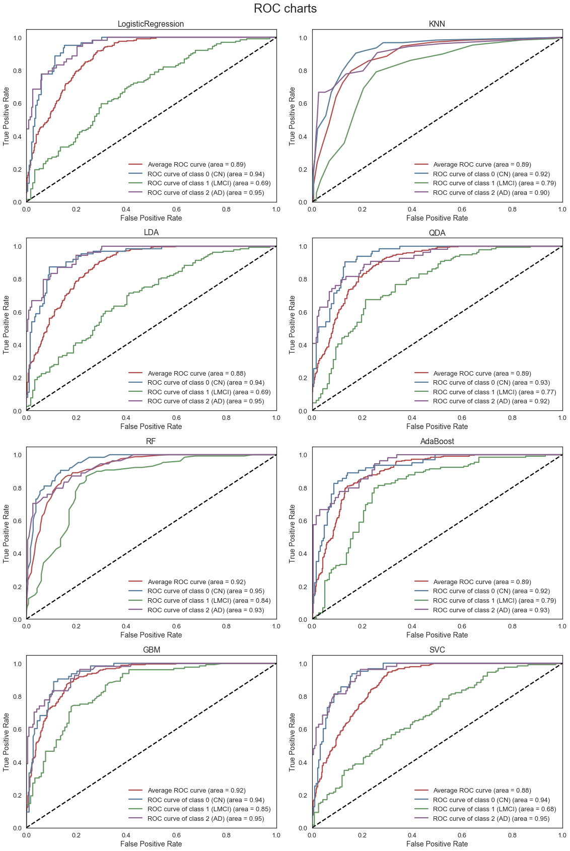
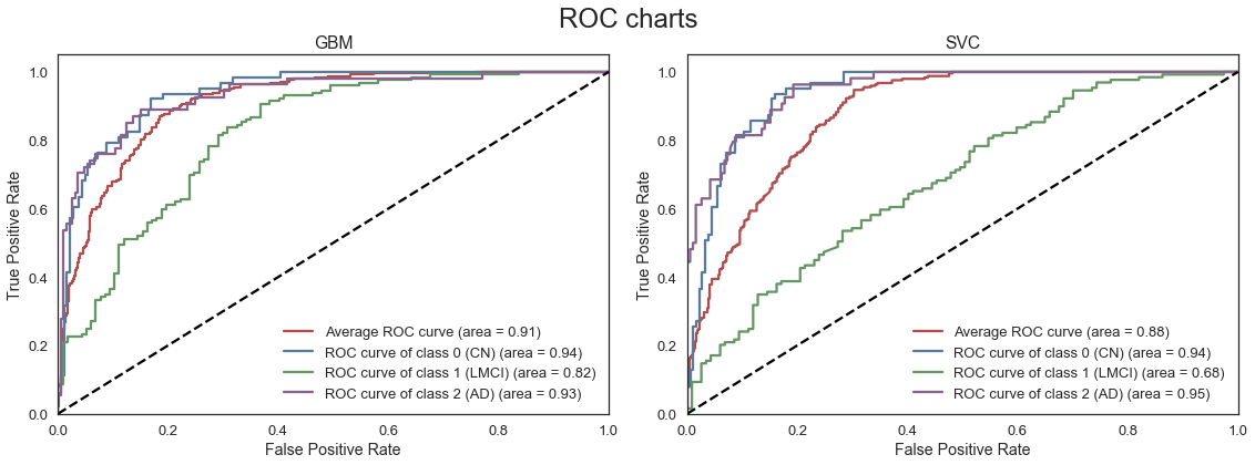
The ROC curves above, describe the trade-off between the True positive rate (TPR) and False Positive Rate (FPR) for each of the models. Models with a higher area under the curve (AUC) or high True Positive Rate for a given False Positive Rate are generally preferred. We note that the RF and GBM models are able to most accurately classify subjects accross all three classes. Although the mean validation accuracy of the LDA model is comparable to the RF and GBM models, the average AUC is lower as the LDA model is less effective at classifying subjects with LMCI.
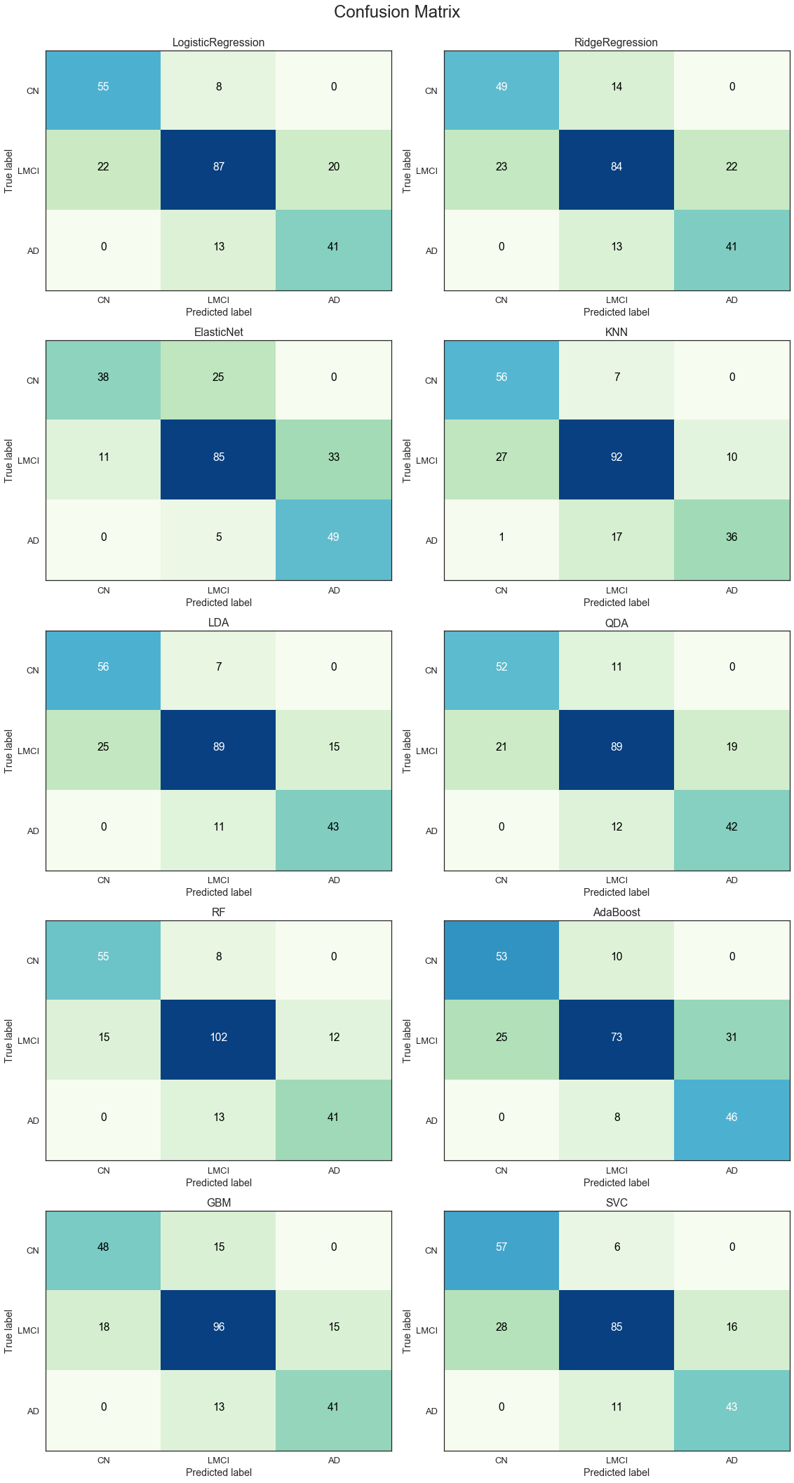
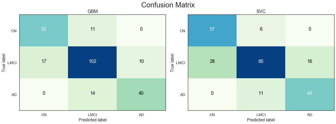
The results from the confusion matrices are consistent with the observations from the ROC curves. The RF and GBM models are the best performers across all three classes on average.
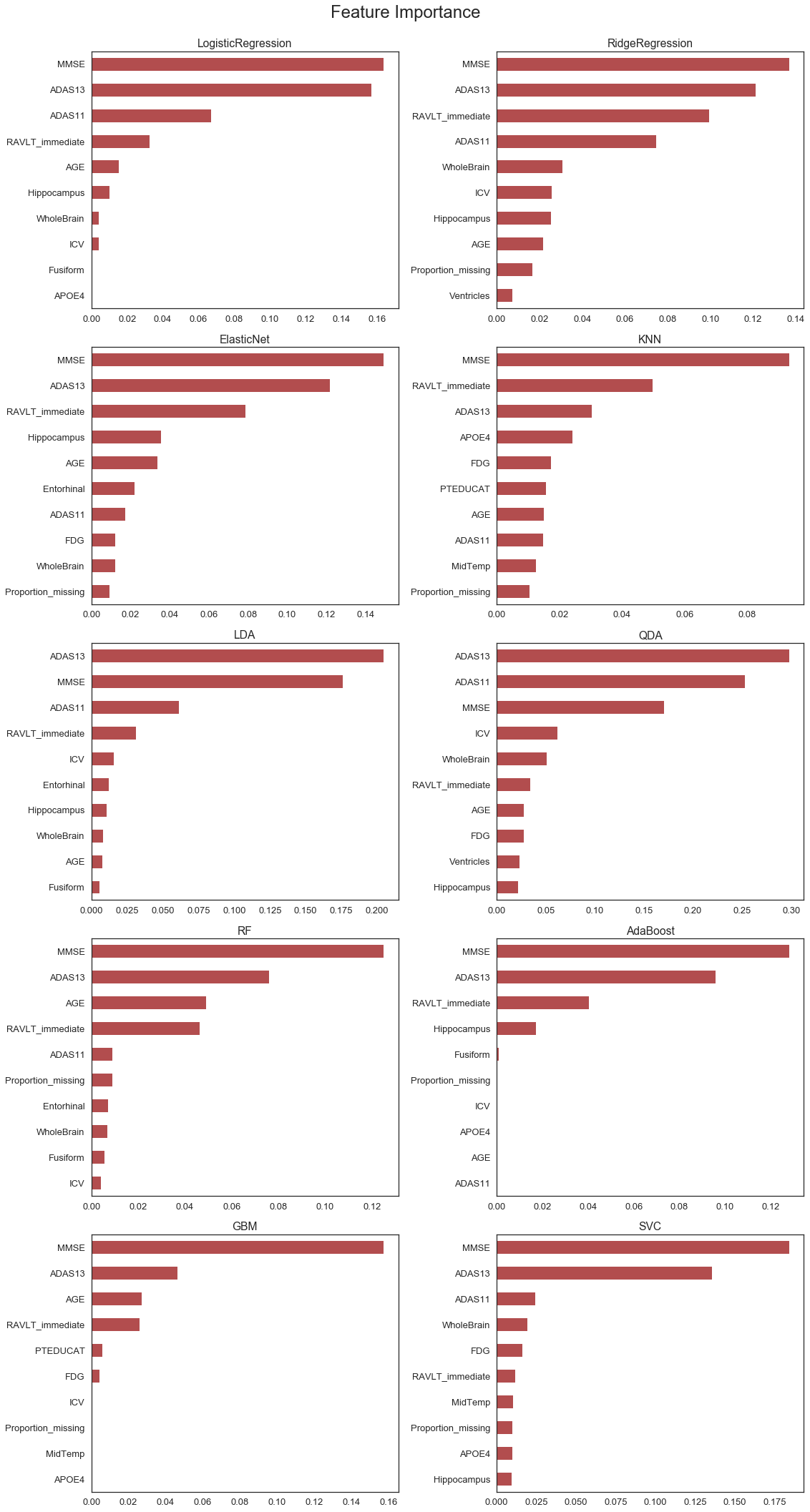
The feature importance plots provide a measure of the relative importance of each of the features included in the model. The plots consistently show that the cognitive tests are the most important features included in the models.
Feature importance measures are typically available for tree-based methods. A bespoke measure was created to compare the importance of features in different model types. The measure is obtained by quantifying the reduction in accuracy after a random shuffle of the obervations for a specific feature. The intuition is that accuracy should reduce significantly for an important feature whereas the effect will be limited for unimportant (random) features. This method would be too computationally intensive for large models with many observations and predictors, but is fit for this exercise.
More parameter tuning for GBM and SVC methods
In this section we conduct more detailed testing of the GBM and SVC methods considering a wider range of model paramters, optimized using cross-validation.
| estimator | min_score | mean_score | max_score | std_score | C | degree | gamma | kernel | learning_rate | max_depth | n_estimators | subsample | |
|---|---|---|---|---|---|---|---|---|---|---|---|---|---|
| 88 | GBM | 0.7143 | 0.7872 | 0.8793 | 0.0536 | - | - | - | - | 0.2 | 5 | 100 | 0.7 |
| 33 | GBM | 0.7368 | 0.7853 | 0.9138 | 0.0564 | - | - | - | - | 0.05 | 3 | 500 | 0.5 |
| 8 | GBM | 0.7321 | 0.7835 | 0.8621 | 0.0451 | - | - | - | - | 0.01 | 3 | 200 | 1 |
| 14 | GBM | 0.7241 | 0.7820 | 0.8448 | 0.0341 | - | - | - | - | 0.01 | 5 | 50 | 1 |
| 24 | GBM | 0.7018 | 0.7819 | 0.8621 | 0.0477 | - | - | - | - | 0.05 | 3 | 50 | 0.5 |
| 5 | GBM | 0.6897 | 0.7819 | 0.8793 | 0.0555 | - | - | - | - | 0.01 | 3 | 100 | 1 |
| 25 | GBM | 0.7069 | 0.7818 | 0.8772 | 0.0536 | - | - | - | - | 0.05 | 3 | 50 | 0.7 |
| 12 | GBM | 0.7193 | 0.7801 | 0.8793 | 0.0467 | - | - | - | - | 0.01 | 5 | 50 | 0.5 |
| 27 | GBM | 0.6667 | 0.7800 | 0.8947 | 0.0623 | - | - | - | - | 0.05 | 3 | 100 | 0.5 |
| 7 | GBM | 0.7193 | 0.7800 | 0.8793 | 0.0446 | - | - | - | - | 0.01 | 3 | 200 | 0.7 |
Mean validation accuracy is slightly improved after extensive parameter tuning.
Full model with all features
Further analysis of the GBM and SVC models based on the full set of predictors.
| estimator | min_score | mean_score | max_score | std_score | C | degree | gamma | kernel | learning_rate | max_depth | n_estimators | subsample | |
|---|---|---|---|---|---|---|---|---|---|---|---|---|---|
| 2 | GBM | 0.7018 | 0.7956 | 0.8966 | 0.0523 | - | - | - | - | 0.01 | 3 | 500 | 0.5 |
| 15 | GBM | 0.7368 | 0.7938 | 0.8966 | 0.0468 | - | - | - | - | 0.05 | 5 | 500 | 1 |
| 13 | GBM | 0.7414 | 0.7937 | 0.8793 | 0.0424 | - | - | - | - | 0.05 | 5 | 200 | 1 |
| 4 | GBM | 0.6842 | 0.7923 | 0.8966 | 0.0663 | - | - | - | - | 0.01 | 5 | 200 | 0.5 |
| 21 | GBM | 0.7091 | 0.7919 | 0.8621 | 0.0482 | - | - | - | - | 0.1 | 5 | 200 | 1 |
| 6 | GBM | 0.6842 | 0.7904 | 0.8793 | 0.0512 | - | - | - | - | 0.01 | 5 | 500 | 0.5 |
| 12 | GBM | 0.7018 | 0.7887 | 0.8793 | 0.0531 | - | - | - | - | 0.05 | 5 | 200 | 0.5 |
| 19 | GBM | 0.7241 | 0.7871 | 0.8276 | 0.0342 | - | - | - | - | 0.1 | 3 | 500 | 1 |
| 20 | GBM | 0.7193 | 0.7871 | 0.8421 | 0.0347 | - | - | - | - | 0.1 | 5 | 200 | 0.5 |
| 11 | GBM | 0.7368 | 0.7870 | 0.8596 | 0.0373 | - | - | - | - | 0.05 | 3 | 500 | 1 |
The table above ranks the best models by mean validation score on the full set of features. We note that the mean accuracy has only improved marginally compared to the smaller set of predictors. This is to some extent expected given the significance of the cognitive test scores, which are all included in the smaller set of predictors. The key MRI and PET measures are also included in the smaller set of predictors. The 400+ additional predictors appears to only include limited additional information, while increasing the dimensionality of the feature space significantly. We note that the GBM model appears to deal better with the large number of predictors that the SVC model.
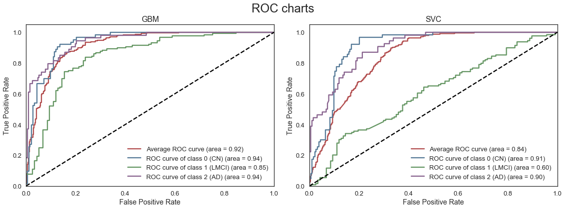
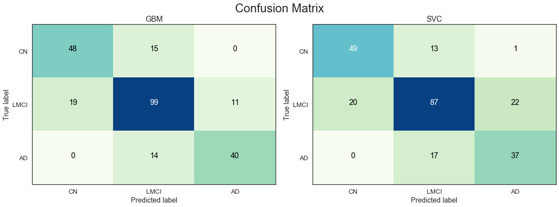
The GBM model appears to have the best predictive performance on the full feature.
XGBoost model
In this section another boosted model is fit using the XGBoost package, that was designed and optimized for boosting trees algorithm. The underlying algorithm of XGBoost is an extension of the classic gradient boosting algorithm. Some of the strenghts of this implementation compared to scikit-learn includes:
Regularization: The algorithm allows for regularization of weights through the lambda and alpha parameters, which helps to reduce over-fitting.
Parallel computing: XGBoost implements parallel processing making it significantly faster on large datasets
Tree pruning: In GBM, a greed algortihm is used that would only stop splitting a node when it encounters a negative loss in the split. XGBoost makes splits up to the maximum depth specified and then prunes the tree backwards to remove redundant splits
| estimator | min_score | mean_score | max_score | std_score | colsample_bytree | learning_rate | max_depth | n_estimators | reg_alpha | subsample | |
|---|---|---|---|---|---|---|---|---|---|---|---|
| 28 | XGBoost | 0.7456 | 0.7817 | 0.8348 | 0.0399 | 1.0 | 0.1 | 5 | 500 | 0.2 | 0.5 |
| 35 | XGBoost | 0.7522 | 0.7783 | 0.8000 | 0.0191 | 1.0 | 0.1 | 7 | 500 | 0.2 | 1.0 |
| 34 | XGBoost | 0.7281 | 0.7766 | 0.8261 | 0.0394 | 1.0 | 0.1 | 7 | 500 | 0.2 | 0.5 |
| 10 | XGBoost | 0.7434 | 0.7765 | 0.8174 | 0.0306 | 0.8 | 0.1 | 5 | 500 | 0.2 | 0.5 |
| 26 | XGBoost | 0.7456 | 0.7748 | 0.8087 | 0.0224 | 1.0 | 0.1 | 5 | 500 | 0.1 | 0.5 |
| 13 | XGBoost | 0.7257 | 0.7747 | 0.8000 | 0.0272 | 0.8 | 0.1 | 7 | 500 | 0.0 | 1.0 |
| 12 | XGBoost | 0.7368 | 0.7731 | 0.8000 | 0.0220 | 0.8 | 0.1 | 7 | 500 | 0.0 | 0.5 |
| 15 | XGBoost | 0.7434 | 0.7730 | 0.8087 | 0.0262 | 0.8 | 0.1 | 7 | 500 | 0.1 | 1.0 |
| 14 | XGBoost | 0.7193 | 0.7730 | 0.8348 | 0.0449 | 0.8 | 0.1 | 7 | 500 | 0.1 | 0.5 |
| 24 | XGBoost | 0.7105 | 0.7729 | 0.8348 | 0.0445 | 1.0 | 0.1 | 5 | 500 | 0.0 | 0.5 |
Test accuracy: 0.78
After determining the optimal parameters of the XGBoost model through cross-validation, the test performance of the model is very comparable to that obtained by the Gradient Boosting model. We note that XGBoost appears to be more computationally efficient, with quicker model fitting and better parallel performance.